Distribution of Speech & Silence Durations (2)
Speech and silence in political speeches again
A "speech activity detector" (SAD) is available on harris, under the appropriate name "sad". This one was written a few years ago by Neville Ryant. Its use is simple, as exemplified below:
    $ sad 010910_WeeklyAddress.wav
    1 out of 1 files successfully segmented.
There are a few optional command-line parameters, notably
      --spch [tsec]     Set min speech dur (default: 0.5 s)
      --nonspch [tsec]  Set min nonspeech dur (default: 0.3 s)
So depending on the quality of the audio and the level of detail we're interesting in, we might instead try something like
     $ sad --spch 0.25 --nonspch 0.15 010910_WeeklyAddress.wav
     1 out of 1 files successfully segmented.
In either case, the result will be a file that looks something like this:
         0.00 0.77 spch
         0.77 1.00 nonspch
         1.00 4.32 spch
         4.32 4.89 nonspch
         4.89 6.11 spch
         [...]
         330.72 331.42 nonspch
         331.42 331.91 spch
         331.91 332.99 nonspch
         332.99 333.58 spch
         333.58 334.35 nonspch
That is, each line has three space-separated fields, namely a start time, and end time, and a label which is either "spch" or "nonspch".
If we want to check the result in Praat, we could run a simple perl script
$ sad2textgrid 010910_WeeklyAddress.lab >010910_WeeklyAddress_sad.TextGrid
and then inspect the audio and textgrid together:

We can merge the SAD TextGrid with the TextGrid from forced alignment to compare them:
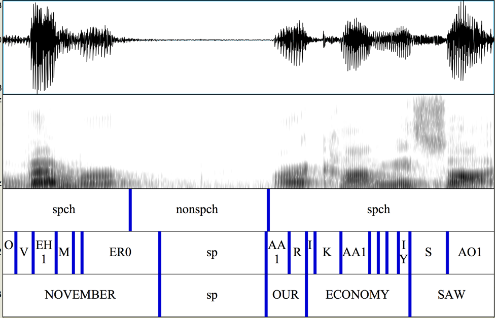
The choices are not exactly the same -- the acoustic models were trained on different materials, etc. -- but we would find that different human annotators would make similarly different choices unless given careful instructions and training.
To compare the overall distributions, let's turn the .word output from the forced aligner into a file in the same format as the SAD output:
$ word2sad 010910_WeeklyAddress.word >010910_WeeklyAddress.lab1
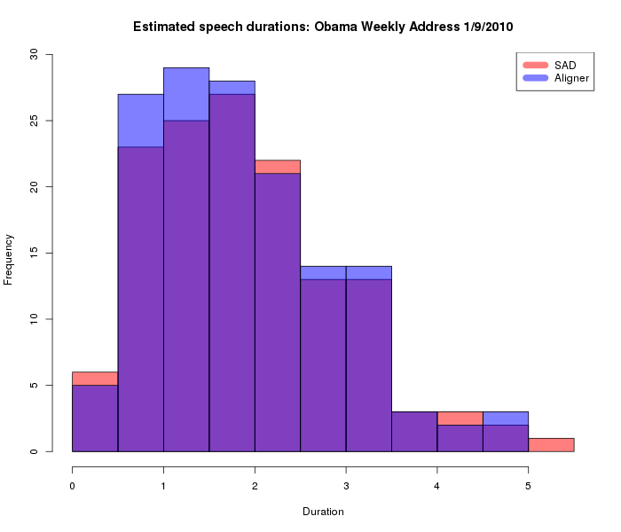
Because these files are simple space-separated text tables, we can read them directly into an R script to compare the results. For the distribution of speech durations, the results are quite similar:
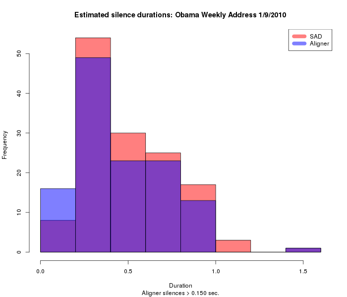
And the distribution of silence durations is also fairly similar, as long as we constrain the aligner in the same way as the SAD program, i.e. to report only silences longer than 150 msec.:
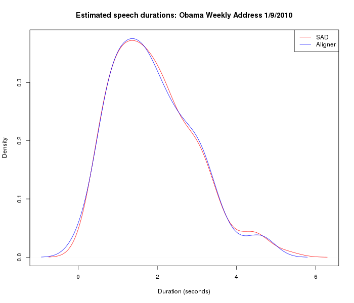
Another way to look at the same thing is as R density plots for speech durations:
And for silence durations:
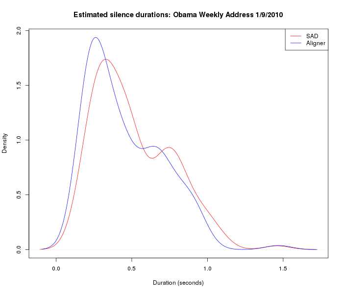
In both the density plots and the histograms, we can see the effect of the SAD program's tendency to find fewer silences, and to estimate their durations as a bit longer. We could make the distributions more similar by adjusting the speech-vs.-silence weight in the SAD program, but for now let's just observe that we need to be careful in comparing such results across categories, to be sure that the effective definition of segmentation is the same, or at least close enough not to introduce a bias.
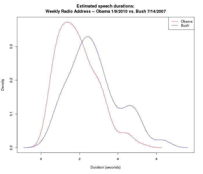
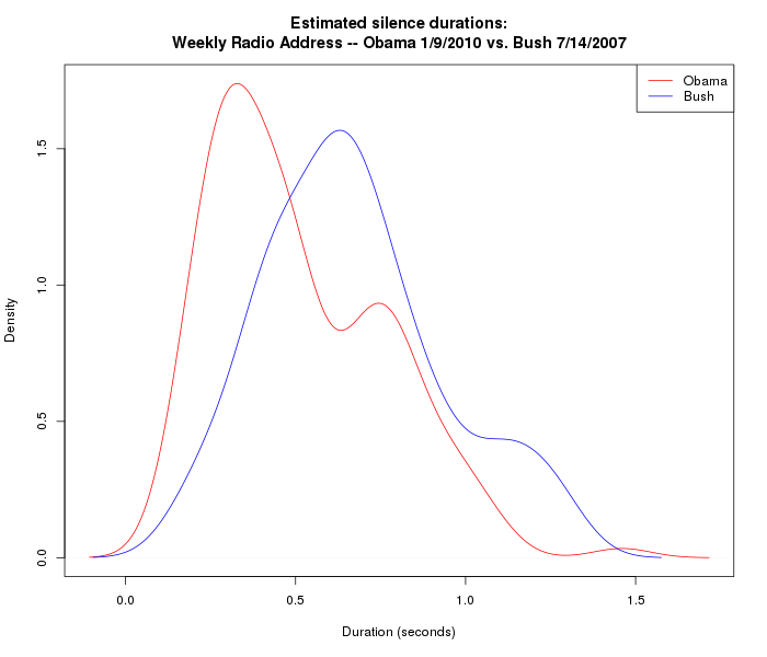
So if we compare weekly radio addresses from two different presidents (Obama 1/9/2010 and Bush 7/14/2007), using the same SAD program with the same parameters (sad --spch 0.25 --nonspch 0.15), we can be fairly confident that we're seeing a difference that's really there in the two men's speech patterns, at least in the two passages analyzed:
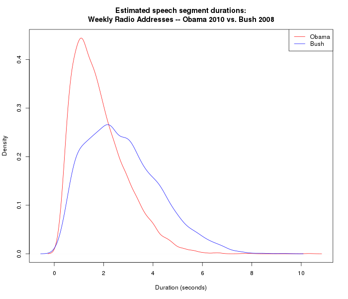
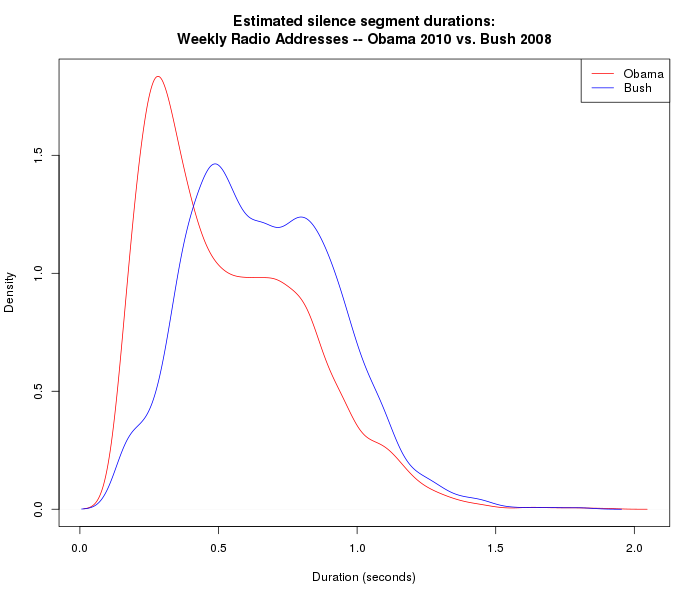
In order to have more confidence that the differences are systematic, we'd want to look at a larger number of similar recordings. So here are the density plots for 48 weekly radio addresses that George W. Bush delivered in 2008, and 50 weekly radio addresses that Barack Obama delivered in 2010:
Alternatively, we can compare the quantiles of the distributions:
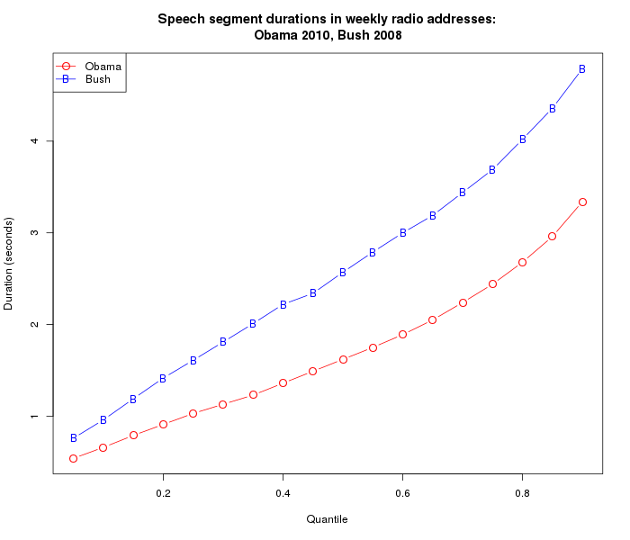

(The R code for the last four plots is here.)
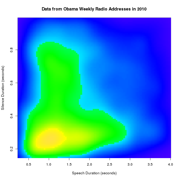
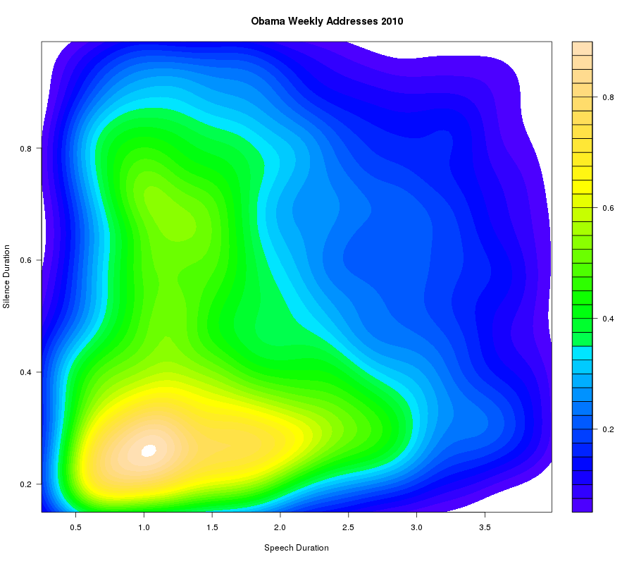
Or again, a 2D density plot -- essentially a smoothed 2D histogram -- of speech-durations vs. immediately following silence-durations, for Obama:
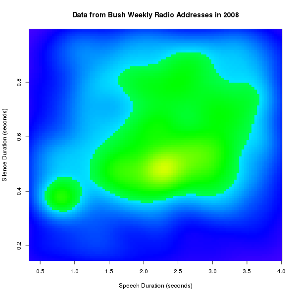
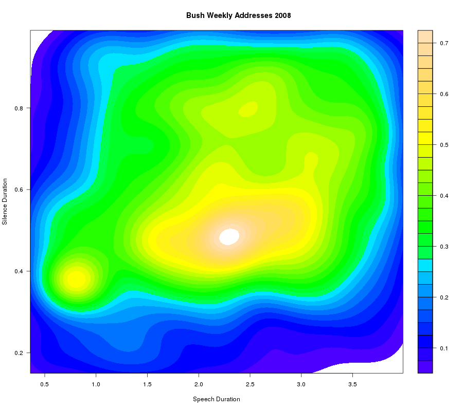
And for Bush:
It may be clearer what's going on if we use R's filled.contour() display function, which shows the boundaries of the levels used in the plot -- where the visually-salient color transitions are essentially arbitrary:
And just for fun, here's the comparable plot for William Carlos Williams' poetry readings at the Library of Congress on May 5, 1945:
